Project Documentation¶

This site provides project documentation. Use the documentation navigation to explore.

How-To Guide¶

Many instructions are common to all our projects.

See ⭐ Workflow: Apply Example to get the example projects running on your machine.

Project Documentation Pages (docs/)¶

• Home - this documentation landing page
• Project Instructions - the standard project workflow
• Your Files - how to copy the example and create your version
• Glossary - project terms and concepts
• API - autogenerated code documentation for the public project interface

Phase 4. Technical Modification¶

I added a constructed feature to my copy of the example notebook:

df_feat["flipper_to_bill"] = df_feat["flipper_length_mm"] / df_feat["bill_length_mm"]

and updated new_cols to include it, so the new feature was reported along with the others.

I chose it because it fit the pattern the example was already demonstrating. The example builds bill_ratio from two bill measurements, so a ratio between a flipper measurement and a bill measurement is the same kind of feature, built from different columns. It is unitless, and it is not derived from the target, so it could not leak body_mass_g.

I verified it by rerunning the notebook and reading the summary log. Before the change, "After features" reported 10 columns against 7 original. After the change it reported 11. The debug sample also printed the new column alongside its inputs, so I could see the values were what I expected rather than trusting the count alone.

Compared with the example, the difference is one additional feature. It is a small change, and it matters mainly as proof that I could add to a working project, rerun it, and explain what moved. It was easy. One line to construct the feature, one line to register it, and the summary reported the result.

Phase 5. Custom Project¶

Basis and Data¶

The example project uses the Seaborn penguins dataset and predicts body_mass_g, a body measurement, from other body measurements. I kept the process and changed the problem.

My dataset is the UCI Student Performance data (Cortez, P. 2014, UCI Machine Learning Repository, https://doi.org/10.24432/C5TG7T, CC BY 4.0), specifically student-mat.csv: 395 students in a secondary school mathematics course at two Portuguese schools, 33 columns covering demographics, family background, social life, school support, and grades. The data is complete, with no missing values in any column.

I chose it because I coordinate a learning center, and the question it raises is one I face: can we tell early which students are heading for a poor outcome, while there is still time to reach them? The limitation worth naming up front is that this is data from two Portuguese secondary schools in 2008. Nothing here transfers directly to my own students.

Modeling Approach¶

This is supervised learning, because the data includes a target. It is a regression problem, because the target is numeric rather than categorical. The example project is also supervised regression, so the approach did not change; the data and the reasoning did.

Module 2 stops before modeling, so no model is fit here. The work is assessing the columns and constructing features.

Target¶

The example target is body_mass_g, a continuous measurement in grams.

My target is G3, the final grade. It is numeric, but unlike body mass it is discrete and bounded: whole numbers from 0 to 20. The order and the spacing are meaningful, so treating it as numeric is reasonable, but it is not continuous, and a regression model could produce a prediction outside the possible range.

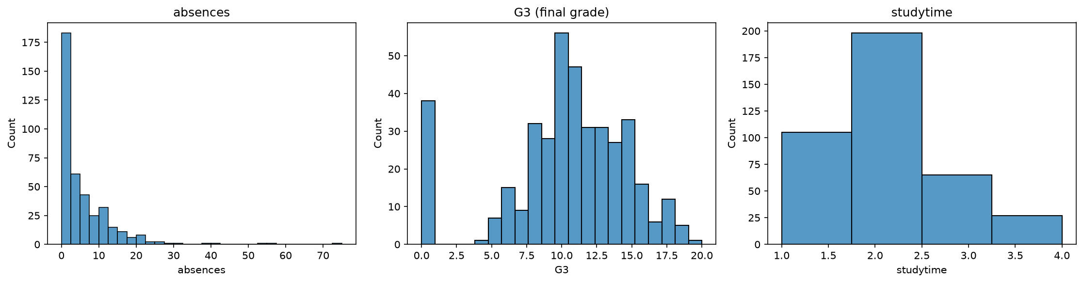
The distribution also has a feature worth noting. Above 5, G3 is roughly bell-shaped. But 38 students score exactly zero, which reads as a separate group rather than the low tail of one distribution. I did not remove or adjust them. A zero final grade is not a data error, and in an early-alert context that student is the point.

Features¶

The example constructs three features from penguin measurements: a ratio (bill_ratio), a rescale (flipper_cm), and a binned category (size_class). It removes nothing.

My project removes two columns and adds two.

G1 and G2, the first and second period grades, are almost certainly the two most predictive columns in the dataset. A model built on them would look very good. But a prediction is only worth making if it arrives while someone can still act on it, and the alert I have in mind comes before the first period grades post. At that point neither column exists. So the two best columns in the data were removed.

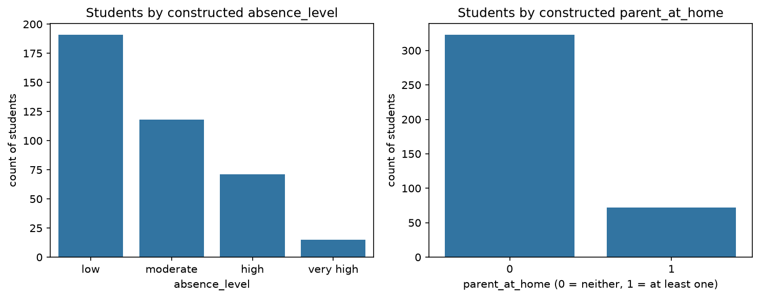
absence_level bins the absence count into four groups, with boundaries at the median (4), the third quartile (8), and the 1.5 IQR upper fence (20), so the cuts come from the distribution. Binning fits a variable where the difference between 0 and 2 absences is noise and the difference between 3 and 30 is a story. The cost is that most students land in "low" and only 15 reach "very high."

parent_at_home flags whether either parent's job is listed as at_home. A parent at home might mean more supervision, or it might mean unemployment and financial strain. Those point in opposite directions and I do not know which one dominates. I built it because the question seemed worth asking.

Neither constructed feature is derived from G3, so neither one leaks the target.

Evaluation and Results¶

The project produced a dataset with the same column count it started with and a different composition: 33 original columns, two removed, two added, 33 after. The summary log reports each step, and the charts show both the distributions that drove the choices and the shape of the features that came out of them.

absence_level groups students into four levels of attendance, with boundaries drawn from the distribution rather than from round numbers. 191 of 395 students land in "low," and 15 land in "very high." parent_at_home flags 72 students with at least one parent whose job is listed as at_home. G1 and G2 are gone, on the grounds that they do not exist when the alert would be sent.

What I cannot report is whether any of it helped. Module 2 ends at feature construction, so there is no model to test these choices against. Every decision documented above is an argument rather than a measurement, and the argument will not be settled until there is something to evaluate it with.

Summary¶

I copied the example notebook, changed the dataset to the UCI Student Performance data, and set G3 as the target. I assessed the columns for type and completeness, looked at the distributions of absences and G3 before deciding anything, removed G1 and G2 on availability grounds, constructed parent_at_home and absence_level, and reported what changed.

What I learned is that the constraint that mattered most had nothing to do with the data quality. The dataset is complete and clean. The thing that shaped every decision was when the prediction needs to arrive, and that is a question about the problem, not about the columns.

The skills here transfer directly to my own work. Any early-alert question at a college runs into the same constraint: some of the strongest predictors of a student's outcome are things you only learn after the point where you could have helped.